How to build a LSTM-based Neural Machine Translation model with fairseq
Neural Machine Translation (NMT) is often an end-to-end pipeline requiring less code and training time compared to Statistical Machine Translation (SMT). Two open-source libraries are often used in this domain: opennmt and fairseq. In this tutorial, we will see how to quickly train a NMT model using LSTM, a type of RNN capable of retaining more information on long range dependencies.
It should be noted that NMT uses often a sequence to sequence model (Seq2Seq), meaning that it takes a sequence of words as inputs, encodes them (encoder) and outputs another sequence of words (decoder). However, the length of the inputs and outputs in NMT needs not to be the same, contrary to tasks like part-of-speech tagging.
RNN, typical use (before attention) and major downside
We mentioned that LSTM was a type of RNN. One of the main drawbacks of the traditional way of using RNN in Seq2Seq (in our case both the encoder and the decoder use LSTMs) is that the encoder transforms a sentence into a single vector (the last hidden state) regardless of the sentence’s length. The state-of-the-art uses the transformer architecture that we will introduce later in another article.
Data preparation
In machine translation, one would typically have a parallel text corpus (also called bitexts) in the following fashion:
Let's try something.\tPermíteme intentarlo.
The \t is the tab separator. Then the whole corpus is separated into two files containing each some monolingual texts. Each text is then filtered to remove sentences containing errors (too long or not good translation) and tokenized (since most models take words as inputs). Then the two separatef files are transformed into a binary format to faciliate training, which can be easily done in fairseq.
The --thresholdtgt and --thresholdsrc options map words appearing less than threshold times to unknown.
fairseq-preprocess \
--source-lang es \
--target-lang en \
--trainpref data/tatoeba.eng_spa.train.tok \
--validpref data/tatoeba.eng_spa.valid.tok \
--testpref data/tatoeba.eng_spa.test.tok \
--destdir data/mt-bin \
--thresholdsrc 3 \
--thresholdtgt 3
Please note that it’s important to specify source and target language because these informations are contained in the filenames. See the structure of the data folder.
[3]:
!tree ./data
./data
├── tatoeba.eng_spa.test.tok.en
├── tatoeba.eng_spa.test.tok.es
├── tatoeba.eng_spa.train.tok.en
├── tatoeba.eng_spa.train.tok.es
├── tatoeba.eng_spa.valid.tok.en
└── tatoeba.eng_spa.valid.tok.es

0 directories, 6 files
Now let’s see the files created by the preprocessing script. Notice the files ended by .bin meaning that it’s a binary format and the two dict files containing all the English/Spanish words in the corpus and their IDs. The two dict files contain 11412 English words and 16828 Spanish words for 200,000 bitext sentences, which is rather expected because there are more verb forms/types in Spanish (conjugation in Spanish is richer).
[17]:
#!bash preprocess.sh
!tree ./data/mt-bin
!head -n 5 ./data/mt-bin/dict.en.txt
!wc -l ./data/mt-bin/dict.en.txt
!wc -l ./data/mt-bin/dict.es.txt
./data/mt-bin
├── dict.en.txt
├── dict.es.txt
├── preprocess.log
├── test.es-en.en.bin
├── test.es-en.en.idx
├── test.es-en.es.bin
├── test.es-en.es.idx
├── train.es-en.en.bin
├── train.es-en.en.idx
├── train.es-en.es.bin
├── train.es-en.es.idx
├── valid.es-en.en.bin
├── valid.es-en.en.idx
├── valid.es-en.es.bin
└── valid.es-en.es.idx

0 directories, 15 files
. 136457
I 43210
the 36227
to 34736
a 25625
   11412 ./data/mt-bin/dict.en.txt
   16828 ./data/mt-bin/dict.es.txt
Training
Let’s kick-start the training process. It’s easy to see from the bash script that we use lstm (default embedding size is 512) as building units, together with the use of adam optimizer and a learning rate of 1.0e-3. max-tokens defines the number of tokens loaded on a single batch.The choice of hyperparameters is a tricky engineering problem better tackled using tensorflow, see for example https://github.com/tensorflow/tensor2tensor#translation. In this tutorial, we will use some random
values. Also note the save-dir option specifying the output path for models. The training would continue infinitely and each time an epoch ends, the checkpoint (model’s parameters) is saved in data/mt-cp. Also, after each epoch, the loss is automatically calculated on the train and val. Whenever you pressed Ctrl-C, the training is stopped. The number of epochs you wait until Ctrl-C is called patience.
[13]:
!cat train.sh
#!bash train.sh
fairseq-train \
data/mt-bin \
--arch lstm \
--share-decoder-input-output-embed \
--optimizer adam \
--lr 1.0e-3 \
--max-tokens 4096 \
--save-dir data/mt-cp
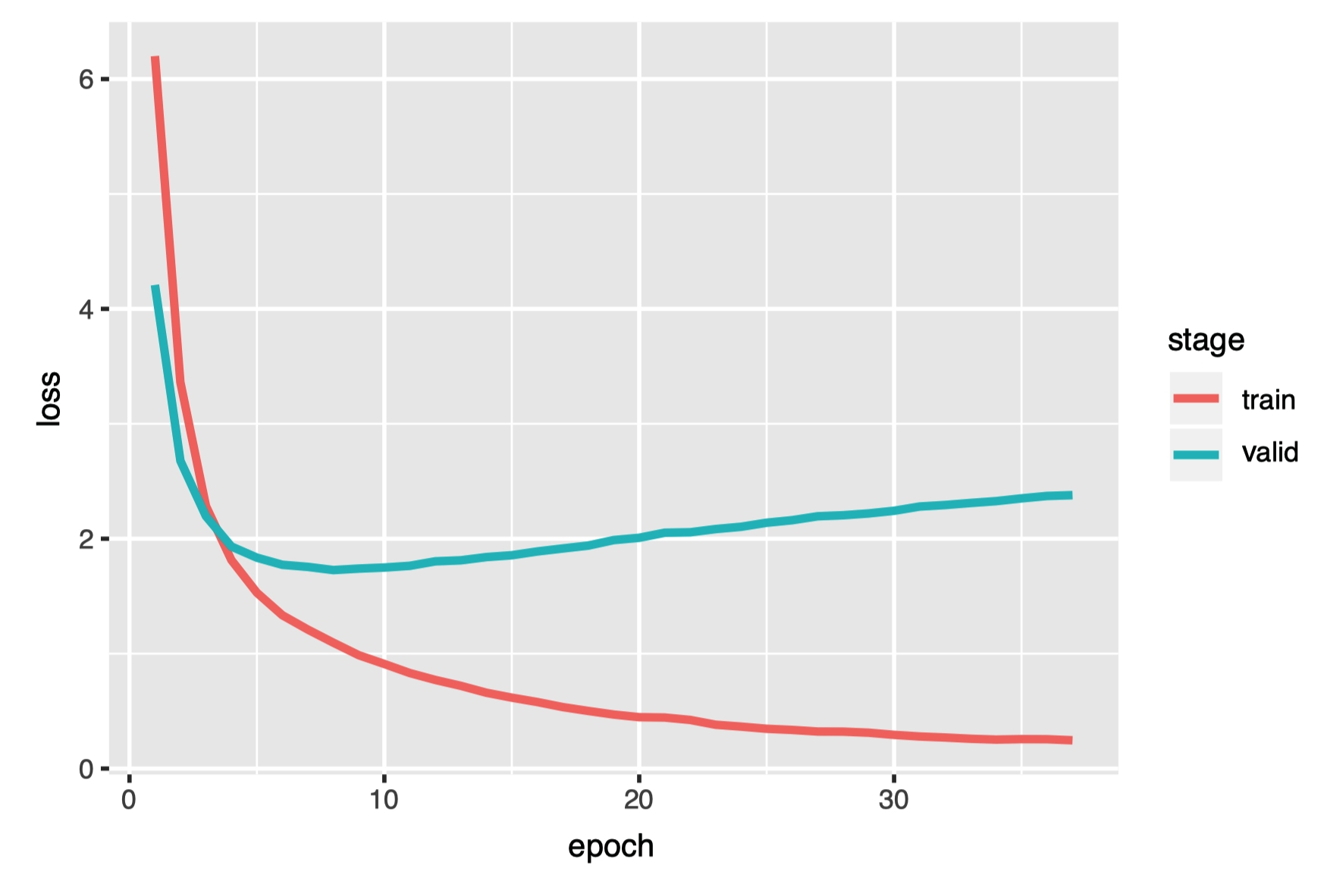
Below is the curve of training and validation loss. This U-shaped curve is very common and the usual practice is to stop the training when validation loss starts to rise (early stopping).
Since training NMT models is very computer-intensive and time-consuming without GPU. I only trained for two epochs on my own machine, resulting in the following folder structure.
[14]:
!tree ./data/mt-pt/
./data/mt-pt/
├── checkpoint1.pt
├── checkpoint2.pt
├── checkpoint_best.pt
└── checkpoint_last.pt

0 directories, 4 files
So how the model is trained?
If one can do some multiclass classification, the term cross entropy should be familiar and it’s a kind of loss used to calculate how a probability distribution p is different from another q (or how p diverges from q or what is the relative entropy of p with respect to q).
More concretely, the decoder takes a <START> token and the last hidden state of the encoder as input and calculate a probability distribution for the next word.
Let’s say the Spanish text is María es hermosa. A hidden state x is generated by the encoder and is feeded into the decoder with a <START> token since it’s the first word. Then the model would compute a probability distribution for each word in the dictionary. Say there are 3 words in the dict: Mary, a, b . The probability calculated by the model would probably be 30%, 40%, 50%. This is obviously wrong, so the model would try to adjust/learn the right distribution based on
the difference between this distribution and the true distribution (cross entropy).
It’s important to note that for the word es, the model would calculate the probability distribution for candidate translations by assuming the previous word is Mary, regardless of the actual distribution. Otherwise it would be very difficult for the model to learn.
Inference/translate
The following script can be used to translate new sentences. Each new sentence occupies a new line in the file source.txt and the translations are redirected to target.txt.
Since the decoder uses the output of the encoder to generate new texts, the model is called conditional language model. Also, it’s a auroregressive model because it always generate text from left to right.
fairseq-interactive --input=source.txt \
data/mt-bin \
--path data/mt-pt/checkpoint_best.pt \
--beam 5 \
--source-lang es \
--target-lang en > target.txt
What is –beam?
There are commonly two ways for the decoder (of translation model) to translate new sentences. Remember that contrary to the training period where the model knows the right translation, the decoder now doesn’t know the right answer for new sentences.
The greedy decoding makes a bold assumption: the quality of the whole translated sentence can be optimized by taking each time the word with the largest score. Let’s say you want to translate the sentence María es hermosa. This means that at each step where a new word is to be translated, the model always select the word with the maximum possibility.
Howeven, this local view can be non ideal. Sometimes you want to consider long-term benefits and it’s exactly the case here because we want a overall good quality at the sentence level. This is the Beam search decoding.
This kind of long-term thinking is prevalent in life. Let’s say that you want to go from A to Z. The first possibility (A-B-C-Z) has the score (1-4-2-2) and the second option (A-D-E-Z) has the score (1-3-4-5). If you take the first itinerary, you are using the greedy decoding because B gives a better score than D (4>3). However, the second option gives a much higher total score (13>9).
We can’t try out every possibility
Since the total words in a dictionary is often huge and it is impossible to test each path possible (for each new word there are n possibilities). It is often necessary to make a compromise and choose a maximum option at each time step (word step for translation). Here we choose 5, meaning that at each new word we choose 5 possible words.
Let’s see the translations :) We use the interactive mode here because the input file is raw text. For binarized data, use fairseq-generate. See here.
A line prefixed with O is a copy of the original source sentence; H is the hypothesis along with an average log-likelihood; D (same as H here), the detokenized hypothesis; and P is the positional score per token position, including the end-of-sentence marker which is omitted from the text. Since the translation of Hola is Hi !, there are 3 positional score for the whole sentence (+end-of-sentence).
[18]:
!cat target.txt
S-0     Hola
W-0     0.052   seconds
H-0     -1.278975486755371      Hi !
D-0     -1.278975486755371      Hi !
P-0     -1.3579 -2.1726 -0.3064
S-1     Me llamo John
W-1     0.048   seconds
H-1     -1.3514807224273682     I 'm called John .
D-1     -1.3514807224273682     I 'm called John .
P-1     -0.3346 -1.4456 -4.4575 -0.7365 -1.1340 -0.0007
S-2     Encantado de conocerte
W-2     0.061   seconds
H-2     -1.2823961973190308     Try to meet you again .
D-2     -1.2823961973190308     Try to meet you again .
P-2     -3.4609 -0.1466 -1.5243 -0.2264 -3.3591 -0.2586 -0.0009
S-3     Últimamente llueve mucho
W-3     0.060   seconds
H-3     -1.3773524761199951     It 's raining a lot of time .
D-3     -1.3773524761199951     It 's raining a lot of time .
P-3     -2.1072 -1.2201 -0.8574 -2.9196 -0.7664 -0.1294 -3.8994 -0.4957 -0.0010
Conclusion, possible improvements and variations
In this tutorial, we go through the whole process of training a NMT model. We use LSTM as building blocks for both the encoder and the decoder. We hope that you can see how simple it is to use fairseq for NMT tasks.
Multiple improvements are however possible, mainly:
Hyperparameter tuning.
More bitexts.
Using other architectures than LSTM-based single embedding approach.
The third point is especially important. As we mentioned in the first section RNN and its major downside, it was usual to encode the whole sentence as a single vector despite the length. So the longer a sentence is, more information would be lost and more difficult it is to translate. For how this issue is tackled, see the following article:
Bahdanau, D., Cho, K., & Bengio, Y. (2016). Neural Machine Translation by Jointly Learning to Align and Translate. ArXiv:1409.0473 [Cs, Stat]. http://arxiv.org/abs/1409.0473
In fact, the lstm option used in fairseq implements already an attention mechanism (technically it’s a form of cross-attention) because the latter is now a de facto standard in machine translation. Later we will see how to use self-attention, an architecture which has literally revolutionized the way to tackle most NLP tasks.
Also, it is very common to rephrase some other NLP tasks as a translation problem, such as:
Chatbot
Question Answering
Grammatical Error Correction
We’ll talk about these different perspectives in other tutorials using other architectures such as Transformer.
Stay tuned :)